Mateusz Hibner

TL;DR

This assignment recreates a full NLP workflow for sentence-level topic classification using the TREC Question Classification dataset. After preparing a clean vocabulary and mitigating OOV issues with a global mean vector initialization, I compared a vanilla RNN, BiLSTM, BiGRU, and CNN. The best classical RNN variant hit 89% test accuracy, while the CNN topped out at 90.2%, highlighting how pretrained embeddings, regularization, and pooling strategies interact. GitHub repo.

1. Introduction

Topic classification assigns predefined intent labels to a question so downstream systems can route or prioritize it. The core idea is simple—map raw text to embeddings, then let a neural model infer its topic—but pulling that off for thousands of noisy, short queries forces us to reason about vocabulary coverage, sequence modeling, and evaluation beyond headline accuracy.

The learning objective for this course project was to turn the semester’s theory into a compare-and-contrast study. I built pipelines that ingest pretrained word embeddings, trained several architectures (RNN, BiLSTM, BiGRU, CNN), quantified how pooling and regularization affect generalization, and documented how different topics benefit from different cues.

2. Preparing Word Embeddings

2.1 Dataset

I worked with the TREC Question Classification dataset (Training set 5 with 5,500 labeled questions). After an 80/20 split with a fixed random seed (42), the test set with 10 held-out questions provided a final checkpoint. Each question belongs to one of six coarse-grained categories:

• ABBR – abbreviation definitions (e.g., “What does AIDS stand for?”)
• DESC – descriptive prompts (e.g., “How did serfdom develop in Russia?”)
• ENTY – entity lookups
• HUM – questions about people
• LOC – geographic targets
• NUM – numeric facts (counts, dates, measurements)

2.2 Vocabulary and preprocessing

Tokenization was handled by spaCy’s en_core_web_sm model. All text was lowercased, two special symbols (<pad>, <unk>) were injected, and I applied a minimum frequency of one so every observed token earned a vocabulary slot. The resulting corpus held 4,361 training questions across 45,591 tokens, yielding a vocabulary of 7,479 entries including specials.

2.3 OOV analysis and mitigation

When mapping tokens to GloVe 6B-100d embeddings, 197 unique words turned out to be OOV, totaling 215 occurrences. Unsurprisingly, categories packed with proper nouns (DESC, ENTY, HUM) drove most of the misses. Instead of random initialization, I computed the global mean vector across all in-vocabulary embeddings and assigned it to every OOV token (and left the embeddings trainable). This centers unknown words in semantic space without biasing the mean with non-lexical tokens.

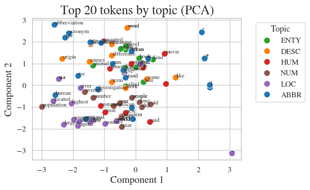
2.4 Semantic clustering

To sanity-check the embedding space, I sampled the 20 most frequent tokens per topic and projected them via PCA. LOC and NUM clusters tightened nicely, signaling coherent semantics, while ABBR, DESC, and HUM points were more diffuse—echoing their lexical variety. Even punctuation such as question marks floated separately, which is expected because they mainly contribute syntactic cues.

3. RNN training & evaluation

3.1 Best configuration

The strongest vanilla RNN used a hidden size of 128, one recurrent layer, dropout of 0.1, and gradient clipping at 1.0. Training ran for 40 epochs with Adam (lr = 1e-3), batch size 64, and max pooling over hidden states. Validation accuracy peaked at 0.853 around epoch 15, while the tiny test set topped out at 0.800.

3.2 Regularization experiments

I swept 49 combinations covering dropout (0.0–0.6), L2 weight decay (0.0–1e-2), gradient clipping, and early stopping. Dropout 0.1 plus weight decay 0.0 and grad_clip=1.0 offered the best validation score (0.841), showing that mild stochastic regularization was enough for this compact dataset.

3.3 Training dynamics

Loss curves dropped quickly over the first ten epochs and then leveled out, so early stopping prevented overfitting once validation loss plateaued. That behavior confirmed the model converged cleanly and did not need aggressive scheduling tricks.

3.4 Pooling strategies

To summarize sequences, I tried max, mean, last hidden state, and attention pooling. Max pooling generalized best by a small margin:

Pooling method	Test accuracy
Max pooling	88.2%
Mean pooling	87.4%
Last hidden state	86.4%
Attention pooling	86.2%

3.5 Topic-wise accuracy

DESC and LOC dominated with 0.97 and 0.93 accuracy respectively—their cues are frequent in the training set. HUM and NUM followed closely (0.89/0.88) thanks to obvious lexical markers such as “who” or “how many.” ENTY and ABBR lagged (0.63/0.78) because they are sparse and contain specialized terminology that GloVe does not always capture.

4. Enhancements

4.1 Bidirectional recurrent models

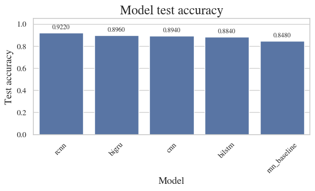
Upgrading the baseline to bidirectional variants paid off immediately. The BiLSTM stacks a forward and backward pass so each prediction considers both preceding and succeeding context, stabilizing gradients with its gating mechanisms. It reached 88.0% test accuracy. The BiGRU trimmed parameters by merging gates yet edged ahead with 89.0%, most likely because the simplified update gate converged faster on this dataset.

4.2 Convolutional neural network

A 1D CNN replaced recurrent passes with kernel banks that capture local n-grams. After convolution + max pooling, a dense head aggregated the most salient phrase-level activations. Besides being easier to parallelize, it booked the best score overall—90.2% test accuracy.

4.3 Further improvements

Two promising next steps are swapping in contextual embeddings (e.g., DistilBERT) to reduce reliance on static GloVe vectors, and augmenting underrepresented classes (ABBR/ENTY) via paraphrasing or back-translation so that the classifier sees more lexical variety during training.

4.4 Topic-focused tuning

Per-class diagnostics suggested specialized thresholds could boost the weakest categories. For example, label-specific loss weighting would penalize ABBR mistakes more, while ontology-driven gazetteers for entities could enrich ENTY representations. Calibrating confidence per class would also help downstream systems decide when to trigger human review.